Pathway case

library(MMRcaseselection)

The pathway was originally proposed by Gerring (2007). He defines the pathway value of a case as \(|resid_{i_{reduced}}-resid_{i_{full}}|\) if it holds that \(|resid_{i_{reduced}}| > |resid_{i_{full}}|\), where ‘full’ stands for the full regression model, ‘reduced’ for the model that lacks the pathway variable of theoretical interest and \(i\) being a case index. Following Gerring, one should only choose among the cases meeting the requirement that \(|resid_{i_{reduced}}| > |resid_{i_{full}}|\). In follow up research, Weller and Barnes (2014) propose a different calculation of the pathway value, \(|resid_{i_{reduced}}|-|resid_{i_{full}}|\), without specifying an additional requirement about the relationship between the full model residuals and reduced model residuals.

The function pathway() calculates both types of pathway values and requires the full regression model and the reduced regression model as input. Both models must be lm objects. The dataframe generated by the function contains all variables from the full model plus the following variables:

full_resid: Residuals in full model
reduced_resid: Residuals in reduced model
pathway_wb: Pathway values as proposed by Weller and Barnes (\(|resid_{i_{reduced}}|-|resid_{i_{full}}|\))
pathway_gvalue: Pathway values as proposed by Gerring (\(|resid_{i_{reduced}}-resid_{i_{full}}|\))
pathway_gstatus: Binary character variable that is coded “yes” if \(|resid_{reduced}| > |resid_{full}|\) is met and “no” otherwise.

df_full <- lm(mpg ~ disp + wt, data = mtcars) # full model
df_reduced <- lm(mpg ~ wt, data = mtcars) # reduced model dropp 'disp' as pathway variable
pw_out <- pathway(df_full, df_reduced) # calculation of pathway variables
head(pw_out)
#>                    mpg disp    wt full_resid reduced_resid  pathway_wb
#> Mazda RX4         21.0  160 2.620  -2.345433    -2.2826106 -0.06282193
#> Mazda RX4 Wag     21.0  160 2.875  -1.490972    -0.9197704 -0.57120172
#> Datsun 710        22.8  108 2.320  -2.472367    -2.0859521 -0.38641476
#> Hornet 4 Drive    21.4  258 3.215   1.785333     1.2973499 -0.48798349
#> Hornet Sportabout 18.7  360 3.440   1.647193    -0.2001440 -1.44704909
#> Valiant           18.1  225 3.460  -1.278631    -0.6932545 -0.58537640
#>                   pathway_gvalue pathway_gtype
#> Mazda RX4             0.06282193            no
#> Mazda RX4 Wag         0.57120172            no
#> Datsun 710            0.38641476            no
#> Hornet 4 Drive        0.48798349            no
#> Hornet Sportabout     1.84733701            no
#> Valiant               0.58537640            no

The visualization of pathway values is different from the presentation of ordinary residuals because two models are involved and an observed-vs-fitted plot is not meaningful. Following the approach by Weller and Barnes, the pathway_xvr() function plots the pathway values against the pathway variable. The option pathwaytype = "pathway_wb produces a plot for the Weller/Barnes values. The pathway variable is determined by the function and does not have to be specified. The plot is a gg object that can be customized with the usual ggplot2 options.

pathway_xvr(df_full, df_reduced, pathway_type = "pathway_wb")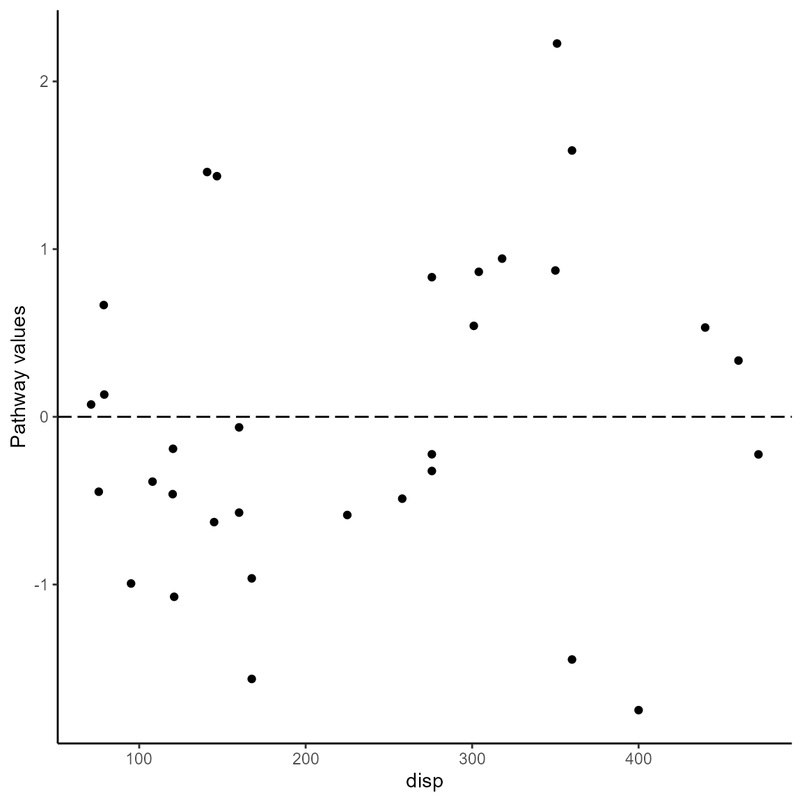

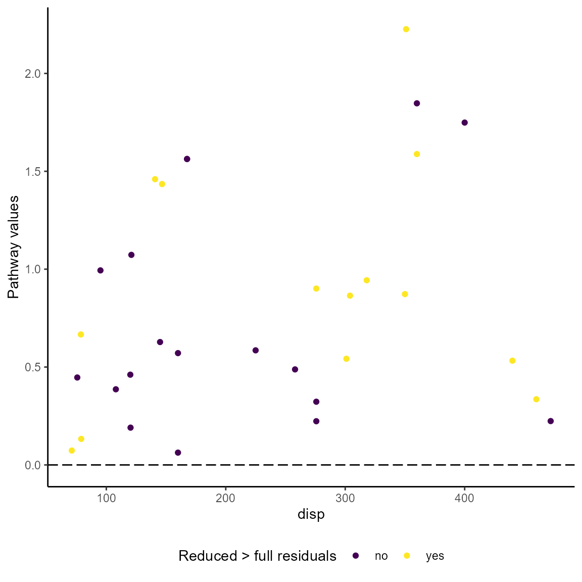
The Gerring pathway values are plotted against the pathway variable if the option is `pathway_type = “pathway_gvalue”. A color scheme is used to distinguish the cases that meet the pathway case requirement (“yes”) from those that don’t (“no”).

pathway_xvr(df_full, df_reduced, pathway_type = "pathway_gvalue")

Ingo Rohlfing

2021-09-28